We want to find out how the numbers in the raw file relate to the exposure that the sensor has received. We can also use the same measurements later to calculate the signal to noise ratio.
We photograph a flat target of uniform reflectance that is evenly illuminated. We use a fixed aperture but vary the shutter speed over a wide range so that we have shots that are heavily under-exposed, heavily over-exposed, and also a fair number at intermediate points. We take two shots at each shutter speed so that we can subtract them later to get the noise.
The EF70-200mm f/2.8L IS lens was used set at 200mm focal length and focussed at infinity, although the target was 1.5m away. For further details of the method please see here.
For ISO 1600, I ended up with 16 pairs of images, each pair taken at a different exposure. The aperture was f/16 and the shutter speeds varied from 1/8000 to 0.4 seconds.
I decided on this occasion to take some additional points at the dark end of the test. As the camera does not have shutter speeds faster than 1/8000 sec, I closed the aperture to f/22 and then f/32, and finally added a Lee 0.6ND (=-2 stop) neutral density filter over the lens. Of course these very small apertures will cause diffraction but I don't think that matters given that we have deliberately defocussed the image anyway. They will also accentuate any dust spots on the sensor but this shouldn't matter when we come to subtract one frame from the other.
The statistics of a 200 x 200 pixel area in the centre of the image for the green wells are in the table below, and you can scroll it down to see figures for the red and blue:
Looking at the Standard Deviation column, it is obvious that for the longest two exposures of the green, and the longest one of the red and blue, the standard deviation is zero. This tells us that the firmware is clipping the numbers in the raw file at 3713, which is 383 short of the maximum output of the camera's 12-bit ADC.
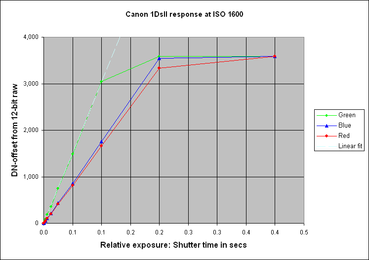
The graph shows the response of all three colours on linear scales, after removing the offset of about 130 that we measured here.
As already mentioned, the fact that the green curve is steeper than the other two may simply be due to the lighting of the target being more intense in the green than the blue region of the spectrum.
The dashed white line is the best straight line fit to the twelve green points whose shutter equivalent speeds are in the range 0.1 to
1/16,000 sec and with the intercept constrained to be zero.
The equation is
DN = 30325.7 * T,
where T is the shutter time in seconds. R² = 0.9998 (Of course, the slope of this line only applies to the
particular target and illumination used. It is done to demonstrate the linearity, see the right-hand two columns of the table above)
For signal values greater than 4 (DN-offset > 4), the RMS nonlinearity is 15.4%.
Because of the linear exposure time scale, many of the data points are crowded in the bottom left corner. A better view is given by plotting the same data on logarithmic scales:
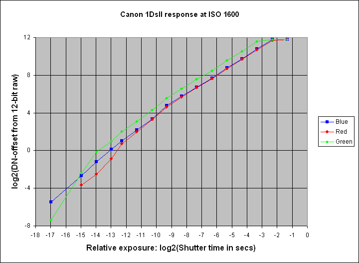
The horizontal axis is relative exposure in photgraphic stops. The offset has been subtracted from the DN values (not that this matters on a log plot). I have suppressed the bottom red point because its mean DN was slightly less than the offset and hence produced a negative figure.
This gives a better impression of the linearity of the camera's response. The range of the linear region can be seen to be about 10.7 stops, although the red fades a bit at the lefthand end. It does not follow that that is the camera's dynamic range, as we shall see later, because we also have to consider the noise.
Peter Facey, Winchester, England
20080311 originated